Wave spectra
[1]:
# Import auxiliary libraries for demonstration

import matplotlib as mpl
import matplotlib.pyplot as plt
import numpy as np
import warnings

plt.rcParams[ "figure.figsize" ] = [ 5, 4 ]

plt.rcParams[ "figure.dpi" ] = 80
plt.rcParams[ "font.family" ] = "Times New Roman"
plt.rcParams[ "font.size" ] = '14'

# Filter the plot warning
warnings.filterwarnings( "ignore" )
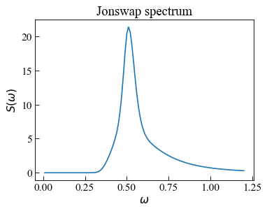
Jonswap Spectrum
The Jonswap spectrum can be expressed,
where \(\omega\) is the wave frequency; \(\omega_p\) is the peak frequency; \(\alpha\) is the intensity of the spectrum, default value = 0.0081; \(\beta\) is the shape factor, default value = 1.25; \(\gamma\) is the peak enhancement factor, default value = 3.3; \(g\) is the acceleration due to gravity, default value = 9.81.
Usually, the input paramters can be determined by the following equation from the JONSWAP experiment,
where \(U_w\) is the wind speed at 10m above the sea surface; \(F\) is the distance from a lee shore.
where \(\omega_p\) is the peak frequency; \(U_w\) is the wind speed at 10m above the sea surface.
Function jonswapSpectrum implements the Jonswap sepctrum.
Reference: * Hasselmann, K., Barnett, T.P., Bouws, E., Carlson, H., Cartwright, D.E., Enke, K., Ewing, J.A., Gienapp, A., Hasselmann, D.E., Kruseman, P. and Meerburg, A., 1973. Measurements of wind-wave growth and swell decay during the Joint North Sea Wave Project (JONSWAP). Ergaenzungsheft zur Deutschen Hydrographischen Zeitschrift, Reihe A.
Function help
[2]:
from ffpack.lsm import jonswapSpectrum
help( jonswapSpectrum )
Help on function jonswapSpectrum in module ffpack.lsm.waveSpectra:

jonswapSpectrum(w, wp, alpha=0.0081, beta=1.25, gamma=3.3, g=9.81)
    JONSWAP (Joint North Sea Wave Project) spectrum is an empirical relationship
    that defines the distribution of energy with frequency within the ocean.

    Parameters
    ----------
    w: scalar
        Wave frequency.
    wp: scalar
        Peak wave frequency.
    alpha: scalar, optional
        Intensity of the Spectra.
    beta: scalar, optional
        Shape factor, fixed value 1.25.
    gamma: scalar, optional
        Peak enhancement factor.
    g: scalar, optional
        Acceleration due to gravity, a constant.
        9.81 m/s2 in SI units.

    Returns
    -------
    rst: scalar
        The wave spectrum density value at wave frequency w.

    Raises
    ------
    ValueError
        If w is not a scalar.
        If wp is not a scalar.

    Examples
    --------
    >>> from ffpack.lsm import jonswapSpectrum
    >>> w = 0.02
    >>> wp = 0.51
    >>> rst = jonswapSpectrum( w, wp, alpha=0.0081, beta=1.25, gamma=3.3, g=9.81 )
Example with default values
[3]:
jsfRange = np.linspace( 0.0, 1.2, num=121 )
[4]:
wp = 0.51
jsfResults = [ jonswapSpectrum( w, wp ) for w in jsfRange ]
[5]:
fig, ax = plt.subplots()

ax.plot( np.array( jsfRange ),
         np.array( jsfResults ) )

ax.tick_params(axis='x', direction="in", length=5)
ax.tick_params(axis='y', direction="in", length=5)
ax.set_ylabel( "$S(\omega)$" )
ax.set_xlabel( "$\omega$" )
ax.set_title( "Jonswap spectrum" )

plt.tight_layout()
plt.show()
Pierson Moskowitz Spectrum
The Pierson Moskowitz spectrum can be expressed,
where \(\alpha\) is the intensity of the spectrum, default value = 0.0081; \(\beta\) is the shape factor, default value = 0.74.
where \(g\) is the acceleration due to gravity, default value = 9.81; \(U_w\) is the wind speed at 19.5m above the sea surface.
Reference:
Pierson Jr, W.J. and Moskowitz, L., 1964. A proposed spectral form for fully developed wind seas based on the similarity theory of SA Kitaigorodskii. Journal of geophysical research, 69(24), pp.5181-5190.
Function help
[6]:
from ffpack.lsm import piersonMoskowitzSpectrum
help( piersonMoskowitzSpectrum )
Help on function piersonMoskowitzSpectrum in module ffpack.lsm.waveSpectra:

piersonMoskowitzSpectrum(w, Uw, alpha=0.0081, beta=0.74, g=9.81)
    Pierson Moskowitz spectrum is an empirical relationship
    that defines the distribution of energy with frequency within the ocean.

    Parameters
    ----------
    w: scalar
        Wave frequency.
    Uw: scalar
        Wind speed at a height of 19.5m above the sea surface.
    alpha: scalar, optional
        Intensity of the Spectra.
    beta: scalar, optional
        Shape factor.
    g: scalar, optional
        Acceleration due to gravity, a constant.
        9.81 m/s2 in SI units.

    Returns
    -------
    rst: scalar
        The wave spectrum density value at wave frequency w.

    Raises
    ------
    ValueError
        If w is not a scalar.
        If wp is not a scalar.

    Examples
    --------
    >>> from ffpack.lsm import piersonMoskowitzSpectrum
    >>> w = 0.51
    >>> Uw = 20
    >>> rst = piersonMoskowitzSpectrum( w, Uw, alpha=0.0081,
    ...                                 beta=1.25, g=9.81 )
Example with default values
[7]:
pmsfRange = np.linspace( 0.0, 1.2, num=121 )
[8]:
Uw = 20
pmsfResults = [ piersonMoskowitzSpectrum( w, Uw ) for w in pmsfRange ]
[9]:
fig, ax = plt.subplots()

ax.plot( np.array( pmsfRange ),
         np.array( pmsfResults ) )

ax.tick_params(axis='x', direction="in", length=5)
ax.tick_params(axis='y', direction="in", length=5)
ax.set_ylabel( "$S(\omega)$" )
ax.set_xlabel( "$\omega$" )
ax.set_title( "Pierson Moskowitz spectrum" )

plt.tight_layout()
plt.show()

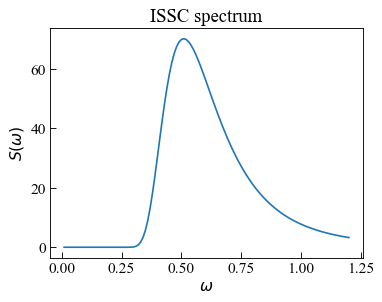
ISSC spectrum
The ISSC spectrum, also known as Bretschneider or modified Pierson-Moskowitz, can be expressed,
where \(\omega\) is the wave frequency; \(\omega_p\) is the peak frequency; \(Hs\) is the significant wave height.
Function isscSpectrum implements the ISSC sepctrum.
Reference:
Guidance Notes on Selecting Design Wave by Long Term Stochastic Method
Function help
[10]:
from ffpack.lsm import isscSpectrum
help( isscSpectrum )
Help on function isscSpectrum in module ffpack.lsm.waveSpectra:

isscSpectrum(w, wp, Hs)
    ISSC spectrum, also known as Bretschneider or modified Pierson-Moskowitz.

    Parameters
    ----------
    w: scalar
        Wave frequency.
    wp: scalar
        Peak wave frequency.
    Hs: scalar
        Significant wave height.

    Returns
    -------
    rst: scalar
        The wave spectrum density value at wave frequency w.

    Raises
    ------
    ValueError
        If w is not a scalar.
        If wp is not a scalar.
        If Hs is not a scalar.

    Examples
    --------
    >>> from ffpack.lsm import isscSpectrum
    >>> w = 0.02
    >>> wp = 0.51
    >>> Hs = 20
    >>> rst = isscSpectrum( w, wp, Hs )
Example with default values
[11]:
isfRange = np.linspace( 0.0, 1.2, num=121 )
[12]:
wp = 0.51
Hs = 20
isfResults = [ isscSpectrum( w, wp, Hs ) for w in isfRange ]
[13]:
fig, ax = plt.subplots()

ax.plot( np.array( isfRange ),
         np.array( isfResults ) )

ax.tick_params(axis='x', direction="in", length=5)
ax.tick_params(axis='y', direction="in", length=5)
ax.set_ylabel( "$S(\omega)$" )
ax.set_xlabel( "$\omega$" )
ax.set_title( "ISSC spectrum" )

plt.tight_layout()
plt.show()
Gaussian Swell spectrum
The Gaussian Swell spectrum is typically used to model long period swell sea, and can be expressed,
where \(\omega\) is the wave frequency; \(\omega_p\) is the peak frequency; \(Hs\) is the significant wave height; \(\delta\) is the peakedness parameter for Gaussian spectral width.
Function gaussianSwellSpectrum implements the ISSC sepctrum.
Reference:
Guidance Notes on Selecting Design Wave by Long Term Stochastic Method
Function help
[14]:
from ffpack.lsm import gaussianSwellSpectrum
help( gaussianSwellSpectrum )
Help on function gaussianSwellSpectrum in module ffpack.lsm.waveSpectra:

gaussianSwellSpectrum(w, wp, Hs, sigma)
    Gaussian Swell spectrum, typically used to model long period
    swell seas [Guidance2016A]_.

    Parameters
    ----------
    w: scalar
        Wave frequency.
    wp: scalar
        Peak wave frequency.
    Hs: scalar
        Significant wave height.
    sigma: scalar
        peakedness parameter for Gaussian spectral width.

    Returns
    -------
    rst: scalar
        The wave spectrum density value at wave frequency w.

    Raises
    ------
    ValueError
        If w is not a scalar.
        If wp is not a scalar.
        If Hs is not a scalar.
        If sigma is not a scalar.

    Examples
    --------
    >>> from ffpack.lsm import gaussianSwellSpectrum
    >>> w = 0.02
    >>> wp = 0.51
    >>> Hs = 20
    >>> sigma = 0.07
    >>> rst = gaussianSwellSpectrum( w, wp, Hs, sigma )

    References
    ----------
    .. [Guidance2016A] Guidance Notes on Selecting Design Wave by Long
       Term Stochastic Method
Example with default values
[15]:
gsfRange = np.linspace( 0.0, 1.2, num=121 )
[16]:
wp = 0.51
Hs = 20
sigma = 0.07
gsfResults = [ gaussianSwellSpectrum( w, wp, Hs, sigma ) for w in gsfRange ]
[17]:
fig, ax = plt.subplots()

ax.plot( np.array( gsfRange ),
         np.array( gsfResults ) )

ax.tick_params(axis='x', direction="in", length=5)
ax.tick_params(axis='y', direction="in", length=5)
ax.set_ylabel( "$S(\omega)$" )
ax.set_xlabel( "$\omega$" )
ax.set_title( "Gaussian Swell spectrum" )

plt.tight_layout()
plt.show()

Ochi-Hubble spectrum
The Ochi-Hubble 6-Parameter spectrum covers shapes of wave spectra associated with the growth and decay of a storm, including swells, and can be expressed,
where \(j = 1, 2\) stands for lower (swell part) and higher (wind seas part) frequency components; \(\omega\) is the wave frequency; \(\omega_p\) is the peak frequency; the six parameters \(H_{s1}, H_{s2}, \omega_{p1}, \omega_{p2}, \lambda_{1}, \lambda_{2}\) are determined numerically to minimize the difference between theoretical and observed spectra.
The modal frequency of the first component, \(\omega_{p1}\), must be less than that of the second, \(\omega_{p2}\). The significant wave height of the first component, \(H_{s1}\), should normally be greater than that of the second, \(H_{s2}\), since most of the wave energy tends to be associated with the lower frequency component.
Function ochiHubbleSpectrum implements the Jonswap sepctrum.
Reference:
Guidance Notes on Selecting Design Wave by Long Term Stochastic Method
Function help
[18]:
from ffpack.lsm import ochiHubbleSpectrum
help( ochiHubbleSpectrum )
Help on function ochiHubbleSpectrum in module ffpack.lsm.waveSpectra:

ochiHubbleSpectrum(w, wp1, wp2, Hs1, Hs2, lambda1, lambda2)
    Ochi-Hubble spectrum covers shapes of wave spectra associated with the growth
    and decay of a storm, including swells. [Guidance2016B]_.

    Parameters
    ----------
    w: scalar
        Wave frequency.
    wp1, wp2: scalar
        Peak wave frequency.
    Hs1, Hs2: scalar
        Significant wave height.
    lambda1, lambda2: scalar

    Returns
    -------
    rst: scalar
        The wave spectrum density value at wave frequency w.

    Raises
    ------
    ValueError
        If w is not a scalar.
        If wp1 or wp2 is not a scalar.
        If Hs1 or Hs2 is not a scalar.
        If lambda1 or lambda2 is not a scalar.
        If wp1 is not smaller than wp2.

    Notes
    -----
    Hs1 should normally be greater than Hs2 since most of the wave energy tends to
    be associated with the lower frequency component.

    Examples
    --------
    >>> from ffpack.lsm import ochiHubbleSpectrum
    >>> w = 0.02
    >>> wp1 = 0.4
    >>> wp2 = 0.51
    >>> Hs1 = 20
    >>> Hs2 = 15
    >>> lambda1 = 7
    >>> lambda2 = 10
    >>> rst = ochiHubbleSpectrum( w, wp1, wp2, Hs1, Hs2, lambda1, lambda2 )

    References
    ----------
    .. [Guidance2016B] Guidance Notes on Selecting Design Wave by Long
       Term Stochastic Method
Example with default values
[19]:
ohfRange = np.linspace( 0.0, 1.2, num=121 )
[20]:
wp1 = 0.4
wp2 = 0.51
Hs1 = 20
Hs2 = 15
lambda1 = 7
lambda2 = 10
ohfResults = [ ochiHubbleSpectrum( w, wp1, wp2, Hs1, Hs2, lambda1, lambda2 )
               for w in ohfRange ]
[21]:
fig, ax = plt.subplots()

ax.plot( np.array( ohfRange ),
         np.array( ohfResults ) )

ax.tick_params(axis='x', direction="in", length=5)
ax.tick_params(axis='y', direction="in", length=5)
ax.set_ylabel( "$S(\omega)$" )
ax.set_xlabel( "$\omega$" )
ax.set_title( "Ochi-Hubble spectrum" )

plt.tight_layout()
plt.show()

Wave spectra comparison
Note:
the shapes of the spectra are sensitive to the parameters
some parameters are fixed in some spectra, and therefore the parameters should be close to the same case
the curves below are adjusted to be similar by trying the parameters
[22]:
waRange = np.linspace( 0.0, 1.2, num=121 )
[23]:
wp = 0.51
jsfResults = [ jonswapSpectrum( w, wp, alpha=0.0081, beta=1.25, gamma=3.3, g=9.81 )
               for w in waRange ]
[24]:
Uw = 25
pmsfResults = [ piersonMoskowitzSpectrum( w, Uw, alpha=0.0081, beta=1.25, g=9.81 )
                for w in waRange ]
[25]:
wp = 0.51
Hs = 12
isfResults = [ isscSpectrum( w, wp, Hs ) for w in waRange ]
[26]:
wp = 0.51
Hs = 12
sigma = 0.025
gsfResults = [ gaussianSwellSpectrum( w, wp, Hs, sigma ) for w in waRange ]
[27]:
fig, ax = plt.subplots( figsize=(10, 4) )

ax.plot( np.array( jsfRange ),
         np.array( jsfResults ),
         label="Jonswap spectrum" )
ax.plot( np.array( pmsfRange ),
         np.array( pmsfResults ),
         label="Pierson Moskowitz spectrum" )
ax.plot( np.array( isfRange ),
         np.array( isfResults ),
         label="ISSC spectrum" )
ax.plot( np.array( gsfRange ),
         np.array( gsfResults ),
         label="Gaussian Swell spectrum" )

ax.tick_params(axis='x', direction="in", length=5)
ax.tick_params(axis='y', direction="in", length=5)
ax.set_ylabel( "$S(\omega)$" )
ax.set_xlabel( "$\omega$" )
ax.set_title( "Wave spectra" )

ax.legend(loc='center left', bbox_to_anchor=(1, 0.5))

plt.tight_layout()
plt.show()
