Wind spectra
[1]:
# Import auxiliary libraries for demonstration

import matplotlib as mpl
import matplotlib.pyplot as plt
import numpy as np
import warnings

plt.rcParams[ "figure.figsize" ] = [ 5, 4 ]

plt.rcParams[ "figure.dpi" ] = 80
plt.rcParams[ "font.family" ] = "Times New Roman"
plt.rcParams[ "font.size" ] = '14'

# Filter the plot warning
warnings.filterwarnings( "ignore" )
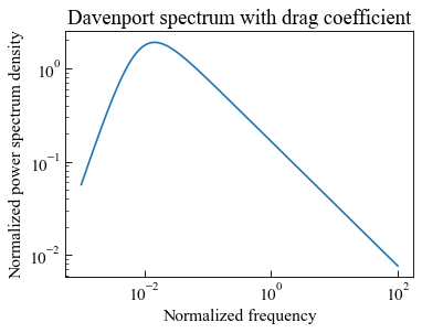
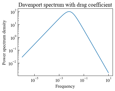
Davenport Spectrum with Drag Coefficient
The Davenport spectrum in the original paper by Davenport can be expressed,
where \(S(n)\) is the power spectrum density ( \(m^2 s^{-2} Hz^{-1}\) ); \(n\) is the frequency; \(\Delta_{1}\) is the velocity ( \(m/s\) ) at standard reference height of 10 \(m\); \(\kappa\) is the drag coefficient referred to mean velocity at 10 \(m\), default value = 0.005.
The normalized power spectrum density is defined as
The normalized frequency is expressed as
The drag coefficient \(\kappa\) is related to the surface type and some recommended values are given as
Type of surface |
\(\kappa\) |
|---|---|
Open unobstructed country (e.g., prairie-type grassland, arctic tundra, desert) |
0.005 |
Country broken by low clustered obstructions such as trees and houses\(^*\) |
0.015 - 0.020 |
Heavilly built-up urban centers with tall buildings |
0.050 |
\(^*\)below 10 \(m\) high
Function davenportSpectrumWithDragCoef implements the Davenport spectrum in the original paper by Davenport.
Reference:
Davenport, A. G. (1961). The spectrum of horizontal gustiness near the ground in high winds. Quarterly Journal of the Royal Meteorological Society, 87(372), 194-211.
Function help
[2]:
from ffpack.lsm import davenportSpectrumWithDragCoef
help( davenportSpectrumWithDragCoef )
Help on function davenportSpectrumWithDragCoef in module ffpack.lsm.windSpectra:

davenportSpectrumWithDragCoef(n, delta1, kappa=0.005, normalized=True)
    Davenport spectrum in the original paper by Davenport [Davenport1961]_.

    Parameters
    ----------
    n: scalar
        Frequency ( Hz ) when normalized=False.
        Normalized frequency when normalized=True.
    delta1: scalar
        Velocity ( m/s ) at standard reference height of 10 m.
    kappa: scalar, optional
        Drag coefficient referred to mean velocity at 10 m.  Default value 0.005
        corresponding to open unobstructed country [Davenport1961]_.
        The recommended value for heavilly built-up urban centers with
        tall buildings is 0.05. The recommended value for country broken by
        low clustered obstructions is between 0.015 and 0.02.
    normalized: bool, optional
        If normalized is set to False, the power spectrum density will be returned.

    Returns
    -------
    rst: scalar
        Power spectrum density ( m^2 s^-2 Hz^-1 ) when normalized=False.
        Normalized power spectrum density when normalized=True.

    Raises
    ------
    ValueError
        If n is not a scalar.
        If delta1 is not a scalar.

    Examples
    --------
    >>> from ffpack.lsm import davenportSpectrumWithDragCoef
    >>> n = 2
    >>> delta1 = 10
    >>> rst = davenportSpectrumWithDragCoef( n, delta1, kappa=0.005,
    ...                                      normalized=True )

    References
    ----------
    .. [Davenport1961] Davenport, A.G., 1961. The spectrum of horizontal gustiness
       near the ground in high winds. Quarterly Journal of the Royal Meteorological
       Society, 87(372), pp.194-211.
Example with default values
[3]:
dsnRange = [ 10**i for i in np.linspace( -3, 2, num=121 ) ]
[4]:
delta1 = 10
dsnResults = [ davenportSpectrumWithDragCoef( n, delta1, normalized=True )
               for n in dsnRange ]
[5]:
fig, ax = plt.subplots()
plt.xscale("log")
plt.yscale("log")

ax.plot( np.array( dsnRange ),
         np.array( dsnResults ) )

ax.tick_params(axis='x', direction="in", length=5)
ax.tick_params(axis='y', direction="in", length=5)
ax.tick_params(axis='x', direction="in", length=3, which='minor')
ax.tick_params(axis='y', direction="in", length=3, which='minor')
ax.set_xlabel( "Normalized frequency" )
ax.set_ylabel( "Normalized power spectrum density" )
ax.set_title( "Davenport spectrum with drag coefficient" )

plt.tight_layout()
plt.show()
[6]:
dsnfRange = [ 10**i for i in np.linspace( -6, 1, num=181 ) ]
[7]:
delta1 = 10
dsnfResults = [ davenportSpectrumWithDragCoef( n, delta1, normalized=False )
                for n in dsnfRange ]
[8]:
fig, ax = plt.subplots()
plt.xscale("log")
plt.yscale("log")

ax.plot( np.array( dsnfRange ),
         np.array( dsnfResults ) )

ax.tick_params(axis='x', direction="in", length=5)
ax.tick_params(axis='y', direction="in", length=5)
ax.tick_params(axis='x', direction="in", length=3, which='minor')
ax.tick_params(axis='y', direction="in", length=3, which='minor')
ax.set_xlabel( "Frequency" )
ax.set_ylabel( "Power spectrum density" )
ax.set_title( "Davenport spectrum with drag coefficient" )

plt.tight_layout()
plt.show()
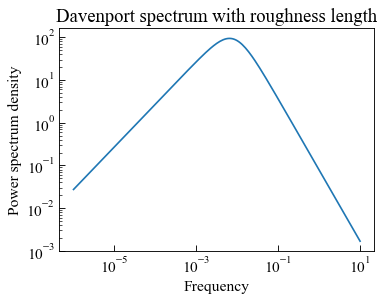
Davenport Spectrum with Roughness Length
The Davenport spectrum in the paper by Hiriart et al. can be expressed,
where \(S(n)\) is the power spectrum density ( \(m^2 s^{-2} Hz^{-1}\) ); \(n\) is the frequency; \(u_{f}\) is the friction velocity ( \(m/s\) ); \(u_{z}\) is the mean wind speed ( \(m/s\) ) measured at height \(z\); \(z\) is the height above the ground, default value = 10 \(m\); \(z_{0}\) is the roughness length, default value = 0.03 \(m\) corresponding to open exposure case in NIST database.
The friction velocity \(u_{f}\) is calculated as
where \(k\) is the von Karman’s constant and \(k=0.4\).
The normalized power spectrum density is defined as
The normalized frequency is expressed as
Function davenportSpectrumWithRoughnessLength implements the Davenport spectrum in the paper by Hiriart et al.
Reference:
Hiriart, D., Ochoa, J. L., & Garcia, B. (2001). Wind power spectrum measured at the San Pedro Mártir Sierra. Revista Mexicana de Astronomia y Astrofisica, 37(2), 213-220.
Ho, T. C. E., Surry, D., & Morrish, D. P. (2003). NIST/TTU cooperative agreement-windstorm mitigation initiative: Wind tunnel experiments on generic low buildings. London, Canada: BLWTSS20-2003, Boundary-Layer Wind Tunnel Laboratory, Univ. of Western Ontario.
Function help
[9]:
from ffpack.lsm import davenportSpectrumWithRoughnessLength
help( davenportSpectrumWithRoughnessLength )
Help on function davenportSpectrumWithRoughnessLength in module ffpack.lsm.windSpectra:

davenportSpectrumWithRoughnessLength(n, uz, z=10, z0=0.03, normalized=True)
    Davenport spectrum in the paper by Hiriart et al. [Hiriart2001]_.

    Parameters
    ----------
    n: scalar
        Frequency ( Hz ) when normalized=False.
        Normalized frequency when normalized=True.
    uz: scalar
        Mean wind speed ( m/s ) measured at height z.
    z: scalar, optional
        Height above the ground ( m ), default to 10 m.
    z0: scalar, optional
        Roughness length ( m ), default to 0.03 m corresponding to open
        exposure case in [Ho2003]_.
    normalized: bool, optional
        If normalized is set to False, the power spectrum density will be returned.

    Returns
    -------
    rst: scalar
        Power spectrum density ( m^2 s^-2 Hz^-1 ) when normalized=False.
        Normalized power spectrum density when normalized=True.

    Raises
    ------
    ValueError
        If n is not a scalar.
        If uz is not a scalar.

    Examples
    --------
    >>> from ffpack.lsm import davenportSpectrumWithRoughnessLength
    >>> n = 2
    >>> uz = 10
    >>> rst = davenportSpectrumWithRoughnessLength( n, uz, z=10, z0=0.03,
    ...                                             normalized=True )

    References
    ----------
    .. [Hiriart2001] Hiriart, D., Ochoa, J.L. and Garcia, B., 2001. Wind power
       spectrum measured at the San Pedro Mártir Sierra. Revista Mexicana de
       Astronomia y Astrofisica, 37(2), pp.213-220.
    .. [Ho2003] Ho, T.C.E., Surry, D. and Morrish, D.P., 2003. NIST/TTU cooperative
       agreement-windstorm mitigation initiative: Wind tunnel experiments on generic
       low buildings. London, Canada: BLWTSS20-2003, Boundary-Layer Wind Tunnel
       Laboratory, Univ. of Western Ontario.
Example with default values
[10]:
dsrnRange = [ 10**i for i in np.linspace( -3, 2, num=121 ) ]
[11]:
uz = 10
dsrnResults = [ davenportSpectrumWithRoughnessLength( n, uz, normalized=True )
                for n in dsrnRange ]
[12]:
fig, ax = plt.subplots()
plt.xscale("log")
plt.yscale("log")

ax.plot( np.array( dsrnRange ),
         np.array( dsrnResults ) )

ax.tick_params(axis='x', direction="in", length=5)
ax.tick_params(axis='y', direction="in", length=5)
ax.tick_params(axis='x', direction="in", length=3, which='minor')
ax.tick_params(axis='y', direction="in", length=3, which='minor')
ax.set_xlabel( "Normalized frequency" )
ax.set_ylabel( "Normalized power spectrum density" )
ax.set_title( "Davenport spectrum with roughness length" )

plt.tight_layout()
plt.show()

[13]:
dsrnfRange = [ 10**i for i in np.linspace( -6, 1, num=181 ) ]
[14]:
uz = 10
dsrnfResults = [ davenportSpectrumWithRoughnessLength( n, uz, normalized=False )
                 for n in dsrnfRange ]
[15]:
fig, ax = plt.subplots()
plt.xscale("log")
plt.yscale("log")

ax.plot( np.array( dsrnfRange ),
         np.array( dsrnfResults ) )

ax.tick_params(axis='x', direction="in", length=5)
ax.tick_params(axis='y', direction="in", length=5)
ax.tick_params(axis='x', direction="in", length=3, which='minor')
ax.tick_params(axis='y', direction="in", length=3, which='minor')
ax.set_xlabel( "Frequency" )
ax.set_ylabel( "Power spectrum density" )
ax.set_title( "Davenport spectrum with roughness length" )

plt.tight_layout()
plt.show()
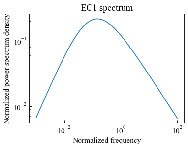
EC1 spectrum
The EC1 spectrum is implemented according to Annex B in BS EN 1991-1-4:2005 Eurocode 1: Actions on structures.
The wind distribution over frequencies is expressed by the non-dimensional power spectral density function \(S_{L}(z,n)\), which should be determined as
where \(S(z,n)\) is the one-sided variance spectrum ( \(m^2 s^{-2} Hz^{-1}\) ); \(f_{L}(z,n)\) is the a non-dimensional frequency determined by the frequency \(n\), the natural frequency in \(Hz\); \(V_{m}\) is the mean velocity ( \(m/s\) ); \(L(z)\) is the turbulence length scale and is determined as
with a reference height of \(z_{t} = 200 \ m\), a reference length scale of \(L_{t} = 300 \ m\), and with \(\alpha = 0.67 + 0.05 ln(z_{0})\), where the roughness length \(z_{0}\) is in \(m\). The minimum height \(z_{min}\) is given in the following table,
Terrain category |
\(z_{0}\) (m) |
\(z_{min}\) (m) |
|---|---|---|
0 Sea or coastal area exposed to the open sea |
0.003 |
1 |
1 Lakes or flat and horizontal area |
0.01 |
1 |
2 Area with low vegetation such as grass and isolated obstacles |
0.05 |
2 |
3 Area with regular cover of vegetation or buildings or with isolated obstacles |
0.3 |
5 |
4 Area in which at least 15 % of the surface is covered with buildings |
1.0 |
10 |
Terrain category |
Description |
|---|---|
0 |
Sea or coastal area exposed to the open sea |
1 |
Lakes or flat and horizontal area with negligible vegetation and without obstacles |
2 |
Area with low vegetation such as grass and isolated obstacles(trees, buildings) with separations of at least 20 obstacle heights |
3 |
Area with regular cover of vegetation or buildings or with isolated obstacles with separations of maximum 20 obstacle heights (such as villages, suburban terrain, permanent forest) |
4 |
Area in which at least 15 % of the surface is covered with buildings and their average height exceeds 15 m |
Function ec1Spectrum implements the spectrum in Eurocode 1.
Reference:
EN1991-1-4, 2005. Eurocode 1: Actions on structures.
Function help
[16]:
from ffpack.lsm import ec1Spectrum
help( ec1Spectrum )
Help on function ec1Spectrum in module ffpack.lsm.windSpectra:

ec1Spectrum(n, uz, sigma=0.03, z=10, tcat=0, normalized=True)
    EC1 spectrum is implemented according to Annex B [EN1991-1-42005]_.

    Parameters
    ----------
    n: scalar
        Frequency ( Hz ) when normalized=False.
        Normalized frequency when normalized=True.
    uz: scalar
        Mean wind speed ( m/s ) measured at height z.
    sigma: scalar, optional
        Standard derivation of wind.
    z: scalar, optional
        Height above the ground ( m ), default to 10 m.
    tcat: scalar, optional
        Terrain category, could be 0, 1, 2, 3, 4
        Default to 0 (sea or coastal area exposed to the open sea) in EC1 Table 4.1.
    normalized: bool, optional
        If normalized is set to False, the power spectrum density will be returned.

    Returns
    -------
    rst: scalar
        Power spectrum density ( m^2 s^-2 Hz^-1 ) when normalized=False.
        Normalized power spectrum density when normalized=True.

    Raises
    ------
    ValueError
        If n is not a scalar.
        If uz is not a scalar.
        If tcat is not int or not within range of 0 to 4

    Examples
    --------
    >>> from ffpack.lsm import ec1Spectrum
    >>> n = 2
    >>> uz = 10
    >>> rst = ec1Spectrum( n, uz, sigma=0.03, z=10, tcat=0, normalized=True )

    References
    ----------
    .. [EN1991-1-42005] EN1991-1-4, 2005. Eurocode 1: Actions on structures.
Example with default values
[17]:
ec1nRange = [ 10**i for i in np.linspace( -3, 2, num=121 ) ]
[18]:
uz = 10
ec1nResults = [ ec1Spectrum( n, uz, normalized=True ) for n in ec1nRange ]
[19]:
fig, ax = plt.subplots()
plt.xscale("log")
plt.yscale("log")

ax.plot( np.array( ec1nRange ),
         np.array( ec1nResults ) )

ax.tick_params(axis='x', direction="in", length=5)
ax.tick_params(axis='y', direction="in", length=5)
ax.tick_params(axis='x', direction="in", length=3, which='minor')
ax.tick_params(axis='y', direction="in", length=3, which='minor')
ax.set_xlabel( "Normalized frequency" )
ax.set_ylabel( "Normalized power spectrum density" )
ax.set_title( "EC1 spectrum" )

plt.tight_layout()
plt.show()
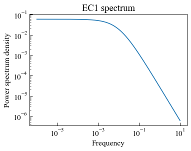
[20]:
ec1nfRange = [ 10**i for i in np.linspace( -6, 1, num=181 ) ]
[21]:
uz = 10
ec1nfResults = [ ec1Spectrum( n, uz, normalized=False ) for n in ec1nfRange ]
[22]:
fig, ax = plt.subplots()
plt.xscale("log")
plt.yscale("log")

ax.plot( np.array( ec1nfRange ),
         np.array( ec1nfResults ) )

ax.tick_params(axis='x', direction="in", length=5)
ax.tick_params(axis='y', direction="in", length=5)
ax.tick_params(axis='x', direction="in", length=3, which='minor')
ax.tick_params(axis='y', direction="in", length=3, which='minor')
ax.set_xlabel( "Frequency" )
ax.set_ylabel( "Power spectrum density" )
ax.set_title( "EC1 spectrum" )

plt.tight_layout()
plt.show()
IEC spectrum
The IEC spectrum is implemented according to IEC 61400-1 (2005), which is a modified version of the Kaimal wind spectrum.
The component power spectral densities are given in non-dimensional form by the equation:
where \(f\) is the frequency in \(Hz\); \(k\) is the index referring to the velocity component direction (i.e. 1 = longitudinal, 2 = lateral, and 3 = upward); \(S_{k}\) is the single-sided velocity component spectrum; \(\sigma_{k}\) is the velocity component standard deviation; \(L_{k}\) is the velocity component integral scale parameter.
The turbulence spectral parameters are given in following table,
\(k = 1\) |
\(k = 2\) |
\(k = 3\) |
|
|---|---|---|---|
Standard deviation \(\sigma_{k}\) |
\(\sigma_{1}\) |
\(0.8\sigma_{1}\) |
\(0.5\sigma_{1}\) |
Integral scale \(L_{k}\) |
\(8.1\Lambda_{1}\) |
\(2.7\Lambda_{1}\) |
\(0.66\Lambda_{1}\) |
where \(\sigma_{1}\) and \(\Lambda_{1}\) are the standard deviation and scale parameters, respectively, of the turbulence. The longitudinal turbulence scale parameter, \(\Lambda_{1}\), at hub height \(z\) shall be given by
The normalized power spectrum density is defined as
The normalized frequency is expressed as
Function iecSpectrum implements the spectrum in IEC 61400-1.
Reference:
IEC, 2005. IEC 61400-1, Wind turbines - Part 1: Design requirements.
Function help
[23]:
from ffpack.lsm import iecSpectrum
help( iecSpectrum )
Help on function iecSpectrum in module ffpack.lsm.windSpectra:

iecSpectrum(f, vhub, sigma=0.03, z=10, k=1, normalized=True)
    IEC spectrum is implemented according to [IEC2005]_.

    Parameters
    ----------
    f: scalar
        Frequency ( Hz ) when normalized=False.
        Normalized frequency when normalized=True.
    vhub: scalar
        Mean wind speed ( m/s ).
    sigma: scalar, optional
        Standard derivation of the turblent wind speed component.
    z: scalar, optional
        Height above the ground ( m ), default to 10 m.
    k: scalar, optional
        Wind speed direction, could be 1, 2, 3
        ( 1 = longitudinal, 2 = lateral, and 3 = upward )
        Default to 1 (longitudinal).
    normalized: bool, optional
        If normalized is set to False, the power spectrum density will be returned.

    Returns
    -------
    rst: scalar
        Single-sided velocity component power spectrum density ( m^2 s^-2 Hz^-1 )
        when normalized=False.
        Normalized single-sided velocity component power spectrum density
        when normalized=True.

    Raises
    ------
    ValueError
        If n is not a scalar.
        If uz is not a scalar.
        If k is not int or not within range of 1 to 3

    Examples
    --------
    >>> from ffpack.lsm import iecSpectrum
    >>> n = 2
    >>> vhub = 10
    >>> rst = iecSpectrum( n, vhub, sigma=0.03, z=10, k=1, normalized=True )

    References
    ----------
    .. [IEC2005] IEC, 2005. IEC 61400-1, Wind turbines - Part 1: Design requirements.
Example with default values
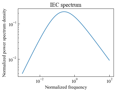
[24]:
icenRange = [ 10**i for i in np.linspace( -3, 2, num=121 ) ]
[25]:
vhub = 10
icenResults = [ iecSpectrum( f, vhub, normalized=True ) for f in icenRange ]
[26]:
fig, ax = plt.subplots()
plt.xscale("log")
plt.yscale("log")

ax.plot( np.array( icenRange ),
         np.array( icenResults ) )

ax.tick_params(axis='x', direction="in", length=5)
ax.tick_params(axis='y', direction="in", length=5)
ax.tick_params(axis='x', direction="in", length=3, which='minor')
ax.tick_params(axis='y', direction="in", length=3, which='minor')
ax.set_xlabel( "Normalized frequency" )
ax.set_ylabel( "Normalized power spectrum density" )
ax.set_title( "IEC spectrum" )

plt.tight_layout()
plt.show()
[27]:
iecnfRange = [ 10**i for i in np.linspace( -4, 2, num=141 ) ]
[28]:
vhub = 10
iecnfResults = [ iecSpectrum( f, vhub, normalized=False ) for f in iecnfRange ]
[29]:
fig, ax = plt.subplots()
plt.xscale("log")
plt.yscale("log")

ax.plot( np.array( iecnfRange ),
         np.array( iecnfResults ) )

ax.tick_params(axis='x', direction="in", length=5)
ax.tick_params(axis='y', direction="in", length=5)
ax.tick_params(axis='x', direction="in", length=3, which='minor')
ax.tick_params(axis='y', direction="in", length=3, which='minor')
ax.set_xlabel( "Frequency" )
ax.set_ylabel( "Power spectrum density" )
ax.set_title( "IEC spectrum" )

plt.tight_layout()
plt.show()

API spectrum
The API spectrum is implemented according to API Recommended practice 2A-WSD (RP 2A-WSD).
The 1 point wind spectrum for the energy density of the longitudinal wind speed fluctuations can be expressed by
where \(n=0.468\); \(f\) is the frequency (\(Hz\)); \(S(f)\) is the spectral energy density at frequency (\(m^2 s^{-2} Hz^{-2}\)); \(z\) is the height above sea level (\(m\)); \(U_{0}\) is the 1 hour mean wind speed at 10 \(m\) above sea level (\(m/s\)).
Function apiSpectrum implements the spectrum in API 2007.
Reference:
API, 2007. Recommended practice 2A-WSD (RP 2A-WSD): Recommnded practice for planning, designing and constructing fixed offshore platforms - working stress design.
Function help
[30]:
from ffpack.lsm import apiSpectrum
help( apiSpectrum )
Help on function apiSpectrum in module ffpack.lsm.windSpectra:

apiSpectrum(f, u0, z=10)
    API spectrum is implemented according to [API2007]_.

    Parameters
    ----------
    f: scalar
        Frequency ( Hz ).
    u0: scalar
        1 hour mean wind speed ( m/s ) at 10 m above sea level.

    Returns
    -------
    rst: scalar
        Power spectrum density ( m^2 s^-2 Hz^-1 ).

    Raises
    ------
    ValueError
        If n is not a scalar.
        If uz is not a scalar.

    Examples
    --------
    >>> from ffpack.lsm import apiSpectrum
    >>> f = 2
    >>> u0 = 10
    >>> rst = apiSpectrum( f, u0 )

    References
    ----------
    .. [API2007] API, 2007. Recommended practice 2A-WSD (RP 2A-WSD):
       Recommnded practice for planning, designing and constructing fixed offshore
       platforms - working stress design.
Example with default values
[31]:
apifRange = [ 10**i for i in np.linspace( -6, 2, num=191 ) ]
[32]:
u0 = 10
apifResults = [ apiSpectrum( f, u0 ) for f in apifRange ]
[33]:
fig, ax = plt.subplots()
plt.xscale("log")
plt.yscale("log")

ax.plot( np.array( apifRange ),
         np.array( apifResults ) )

ax.tick_params(axis='x', direction="in", length=5)
ax.tick_params(axis='y', direction="in", length=5)
ax.tick_params(axis='x', direction="in", length=3, which='minor')
ax.tick_params(axis='y', direction="in", length=3, which='minor')
ax.set_xlabel( "Frequency" )
ax.set_ylabel( "Power spectrum density" )
ax.set_title( "API spectrum" )

plt.tight_layout()
plt.show()

Wind spectra comparison
[34]:
wdRange = [ 10**i for i in np.linspace( -3, 2, num=121 ) ]
[35]:
delta1 = 10
dsnResults = [ davenportSpectrumWithDragCoef( n, delta1, normalized=True )
               for n in wdRange ]
[36]:
uz = 10
dsrnResults = [ davenportSpectrumWithRoughnessLength( n, uz, normalized=True )
                for n in wdRange ]
[37]:
uz = 10
ec1nResults = [ ec1Spectrum( n, uz, normalized=True ) for n in wdRange ]
[38]:
vhub = 10
icenResults = [ iecSpectrum( f, vhub, normalized=True ) for f in wdRange ]
[39]:
fig, ax = plt.subplots( figsize=(10, 4) )
plt.xscale("log")
plt.yscale("log")

ax.plot( np.array( dsnRange ),
         np.array( dsnResults ),
         label="Davenport spectrum with drag coefficient" )
ax.plot( np.array( dsrnRange ),
         np.array( dsrnResults ),
         label="Davenport spectrum with roughness length" )
ax.plot( np.array( ec1nRange ),
         np.array( ec1nResults ),
         label="EC1 spectrum" )
ax.plot( np.array( icenRange ),
         np.array( icenResults ),
         label="IEC spectrum" )


ax.tick_params(axis='x', direction="in", length=5)
ax.tick_params(axis='y', direction="in", length=5)
ax.tick_params(axis='x', direction="in", length=3, which='minor')
ax.tick_params(axis='y', direction="in", length=3, which='minor')
ax.set_xlabel( "Normalized frequency" )
ax.set_ylabel( "Normalized power spectrum density" )
ax.set_title( "Wind spectra" )

ax.legend(loc='center left', bbox_to_anchor=(1, 0.5))

plt.tight_layout()
plt.show()
